It can be a big help if your data in Excel is easy to read (avoiding errors in calculations and or data analysis). I know there are more ways than one to achieve that goal, in this article I’ll show you some code that handles the solution without using conditional formatting. It’s a rough and simple solution…
Sometimes one has to do a lot of mouse clicking… By repetitive clicking and small movements of your hands and other joints you could end up with some nasty RSI (Repetitive Strain Injury) and that ain’t worth it!!! So beat RSI (or your enemy while gaming) by using VBA and Excel to automate some excessive mouse clicks!
In this period of the year most of us are starting to make plans for next year, Excel is an incedibly powerfull tool that can help you visualize your plans. Using Excel’s conditional formatting you can colorize the weekends and make them standout more than the other days of the week or vice versa. This article is an How to colorize the weekends in Excel using conditional formatting.
To colorize the weekends in Excel using conditional formatting, based upon the date in column B, you can use the following formula:
=IF(OR(WEEKDAY($B2)=1;WEEKDAY($B2)=7);1;0)
To create a rule using conditional formatting:
Select the cells that you want to apply the conditional formatting to.
Click “Conditional Formatting”.
Choose “New Rule”.
In the “New Formatting Rule” dialog box, choose “Use a formula”.
Under “Format values”, type the formula: =IF(OR(WEEKDAY($B2)=1;WEEKDAY($B2)=7);1;0)
The formula uses the dates in column B (You can select your own column with dates, by replacing the $B2 part in the formula with the column letter of your choice).
Click “Format”.
In the “Color” box, select your favourite color.
Click “OK” until all dialog boxes are closed.
Suggestions for improving this article are welcome, please let me know and drop me a line.
Did you ever need to rearrange or reorganize columns across multiple sheets in a certain order based on column headers? In this article, I’ll try to explain how to rearrange columns in Excel based on column header information by using Visual Basic for Applications (VBA).
As mentioned in the intro, this article is about rearranging columns in Excel using column header information.
To make it more visible see the images below…
In this example the headers are in alpabetical order: Address, City, Country, Date of Birth, First Name, Last Name, Middle Name, Phone Number, Postal (ZIP) Code, State.
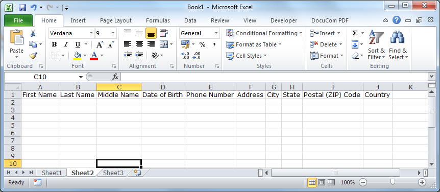
And let’s say you want to change the column order to: First Name,Last Name, Middle Name, Date of Birth, Phone Number,Address, City, State, Postal (ZIP) Code, Country (see the image below)
For those of you that are not familiar with VBA / macro’s use the steps below…
First make sure you’ve got the “Developer” tab in Excel
You might want to use your own headers and ordering, so change the code there 😉
Save your Excel !!!
Press ALT + F8 and Run the Macro
Sub MoveColumns() ‘ MoveColumns Macro ‘ ‘ Developer: Winko Erades van den Berg ‘ E-mail : winko at winko-erades.nl ‘ Developed: 03-10-2011 ‘ Modified: 03-10-2011 ‘ Version: 1.0 ‘ ‘ Description: Rearrange columns in Excel based on column headerDim iRow As Long Dim iCol As Long’Constant values data_sheet1 = InputBox(“Specify the name of the Sheet that needs to be reorganised:”) ‘Create Input Box to ask the user which sheet needs to be reorganised target_sheet = “Final Report” ‘Specify the sheet to store the results iRow = Sheets(data_sheet1).UsedRange.Rows.Count ‘Determine how many rows are in use’Create a new sheet to store the results Worksheets.Add.Name = “Final Report”
‘Start organizing columns For iCol = 1 To Sheets(data_sheet1).UsedRange.Columns.Count
‘Sets the TargetCol to zero in order to prevent overwriting existing targetcolumns TargetCol = 0
‘Read the header of the original sheet to determine the column order If Sheets(data_sheet1).Cells(1, iCol).Value = “First Name” Then TargetCol = 1 If Sheets(data_sheet1).Cells(1, iCol).Value = “Middle Name” Then TargetCol = 2 If Sheets(data_sheet1).Cells(1, iCol).Value = “Last Name” Then TargetCol = 3 If Sheets(data_sheet1).Cells(1, iCol).Value = “Date of Birth” Then TargetCol = 4 If Sheets(data_sheet1).Cells(1, iCol).Value = “Phone Number” Then TargetCol = 5 If Sheets(data_sheet1).Cells(1, iCol).Value = “Address” Then TargetCol = 6 If Sheets(data_sheet1).Cells(1, iCol).Value = “City” Then TargetCol = 7 If Sheets(data_sheet1).Cells(1, iCol).Value = “State” Then TargetCol = 8 If Sheets(data_sheet1).Cells(1, iCol).Value = “Postal (ZIP) Code” Then TargetCol = 9 If Sheets(data_sheet1).Cells(1, iCol).Value = “Country” Then TargetCol = 10
‘If a TargetColumn was determined (based upon the header information) then copy the column to the right spot If TargetCol <> 0 Then ‘Select the column and copy it Sheets(data_sheet1).Range(Sheets(data_sheet1).Cells(1, iCol), Sheets(data_sheet1).Cells(iRow, iCol)).Copy Destination:=Sheets(target_sheet).Cells(1, TargetCol) End If
Next iCol ‘Move to the next column until all columns are read
End Sub
Additional information 1
Someone sent me an alternative solution for reorganizing columns in Excel. The script makes use of the array function in Excel. It does a really nice job but beware, the code handles your data in a way that it does keep your original data structure.
Sub Reorganize_columns() ‘ Reorganize Columns Macro ‘ ‘ Developer: If you want to know, please contact Winko Erades van den Berg ‘ E-mail : winko at winko-erades.nl ‘ Developed: 11-11-2013 ‘ Modified: 11-11-2013 ‘ Version: 1.0 ‘ ‘ Description: Reorganize columns in Excel based on column headerDim v As Variant, x As Variant, findfield As Variant Dim oCell As Range Dim iNum As Long v = Array(“First Name”, “Middle Name”, “Last Name”, “Date of Birth”, “Phone Number”, “Address”, “City”, “State”, “Postal (ZIP) Code”, “Country”) For x = LBound(v) To UBound(v) findfield = v(x) iNum = iNum + 1 Set oCell = ActiveSheet.Rows(1).Find(What:=findfield, LookIn:=xlValues, LookAt:=xlWhole, SearchOrder:=xlByRows, SearchDirection:=xlNext, MatchCase:=False, SearchFormat:=False)If Not oCell.Column = iNum Then Columns(oCell.Column).Cut Columns(iNum).Insert Shift:=xlToRight End If Next x End Sub
Additional information 2
Dennis Klenner from D&R Design Ltd wanted you to know “Header names are case sensitive”! Thank you for the remark Dennis 🙂
Suggestions for improving this article are welcome, please let me know and drop me a line .


You must be logged in to post a comment.